In an hypothesis test, a significance level, alpha, is set for the test and the hypothesis is rejected or not rejected based on whether the test statistic is greater than or less than a value for which the probability of observing a value of the test statistic greater than that value under the null hypothesis is alpha. If we create a random variable, X, which takes on the value 0 in the fail to reject region and the value 1 in the reject region, then the expected value of X under the null hypothesis is alpha and X has a Bernoulli distribution.
If we let Y be the number of trials before getting a significant result, then Y has a geometric distribution, since X has a Bernoulli distribution (see Statistical Distributions, 2nd ed., Evans, Hastings, and Peacock, Wiley, 1993, pp.82-84 or any book on statistical distributions). The number of trials including the first significant event is Y+1. The expected value of a variate from the geometric distribution is one minus alpha divided by alpha:
E(Y) = (1-alpha)/alpha
For example, if alpha equals 0.05, then the expected value of Y is 19 experiments.
However, the negative binomial is a highly skewed distribution, monotonically decreasing as the number of trials increases. The cumulative distribution function for the geometric distribution is [one minus ((one minus alpha) to the (Y plus one))], that is:
F(Y) = 1.0 – (1.0 – alpha)^(Y+1.0)
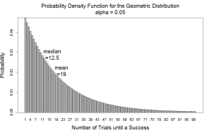
If Y is 19, then the probability of observing an n less than or equal to 20 for the first instance of a false positive is (1.0 – 0.95^20) or 0.64. See the figure below for the distribution of Y given alpha is 0.05.
For skewed distributions, the usual measure of central tendency is the median rather than the mean. The median of a distribution is that value for which the cumulative distribution function equals 0.50. Solving the cumulative distribution function for n, the median number of trials before a success, we get:
1.0 – (1.0 – alpha)^(n + 1) = 0.5
0.5 = (1.0 – alpha)^(n + 1)
ln(0.5) = (n + 1) ln(1.0 – alpha)
n = ln(0.5) / ln(1.0 – alpha) – 1.0
For alpha equal to 0.05, n equals 12.5, which can be rounded down to 12.
We are used to working with the expected value of X, alpha. To convert the median of Y to an alpha level, we can find the value of alpha for which the median of Z is the expected value of Y, where Z is also distributed geometrically. That is:
E(Y) = ln(0.5) / ln(1.0 – alpha) – 1.0
ln(1.0 – alpha) = ln(0.5) / (E(Y) + 1.0)
1.0 – alpha = 0.5^(1.0 / (E(Y) + 1.0))
alpha = 1.0 – 0.5^(1.0 / (E(Y) + 1.0))
For E(Y) equal to 19, alpha equals 0.034, so if alpha equals 0.034, the expected value of the test, X, is 0.034 and the median of the reciprocal of the test, Z, is 19. With the median equal to 19, the probability of seeing the first instance of a false positive of a test in less than or equal to 20 trials is now 0.5, which is what is desired.
Some values for median alphas are:
Mean alpha Median alpha
0.100 0.067
0.050 0.034
0.025 0.017
0.010 0.007
For example, for an 0.010 level median alpha test, you would reject the null hypothesis for p-values less than 0.067.
