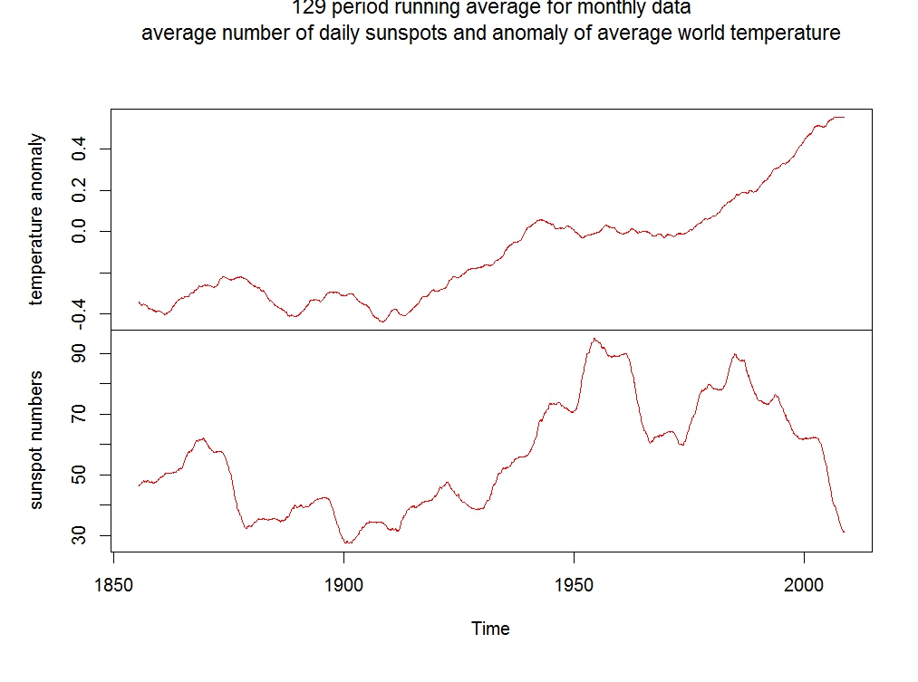
I have found the source of my temperature anomaly data – at Berkeley Earth – the data is the monthly global average temperature data for land and ocean, http://berkeleyearth.org/data. It took several hours of searching.
In my first graph of this blog I plot the graph of the last blog using a period of 129 months for the sunspot cycle. To choose the period, I used the F test from Fuller’s Introduction to Time Series, 1976, Wiley, p.282 to compare different periods close to 132. The period of 129 had the largest F value. The period is 10 years and 9 months.
The second graph I put up is of two plots. The first plot is of the temperature anomaly shown above along with a curve of predicted values, where the predictions are from the model generated by the regression of the 88th through 922th observations of the temperature anomaly vector on the 1st through the 835th observations of the sunspot vector. The model has the largest R squared of the several hundred single variable lag models at which I looked. The best fitting model was for a lag of 87 months fitting 835 observations.

The second plot is the difference between the two curves in the first plot.
This is a very simple model. I was surprised by the drop in the differences in the 1950’s and early 1960’s, but the trend is of an increasing difference as time goes on.
